Linear Regression
Linear regression is a statistical method that tries to show a relationship between variables. It looks at different data points and plots a trend line. Linear regression attempts to model the relationship between two variables by fitting a linear equation to observed data. One variable is considered to be an explanatory variable, and the other is considered to be a dependent variable. For example, a modeler might want to relate the weights of individuals to their heights using a linear regression model. Simply stated, the goal of linear regression is to fit a line to a set of points. When the target variable that we’re trying to predict is continuous, we call the learning problem a regression problem.
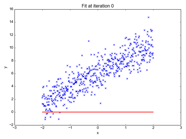
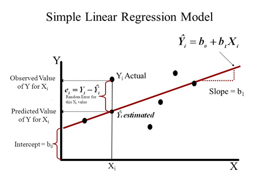
Let’s suppose we want to model the above set of points with a line. To do this we’ll use the standard y = mx + b line equation where m is the line’s slope and b is the line’s y-intercept. To find the best line for our data, we need to find the best set of slope m and y-intercept b values.
Hypothesis
To describe the supervised learning problem slightly more formally, our goal is, given a training set, to learn a function h : X → Y so that h(x) is a “good” predictor for the corresponding value of y. For historical reasons, this function h is called a hypothesis.
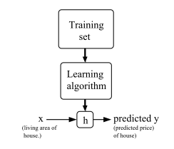
To perform supervised learning, we must decide how we’re going to represent functions/hypotheses h in a computer. As an initial choice, let’s say we decide to approximate y as a linear function of x:
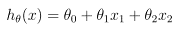
Here, the θ i ’s are the parameters (also called weights)
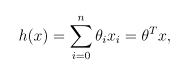
where on the right-hand side above we are viewing θ and x both as vectors, and here n is the number of input variables.
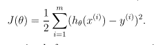
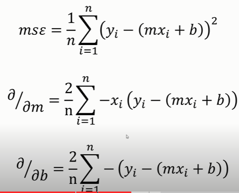
Cost function: LMS (Least Mean Squared) Error
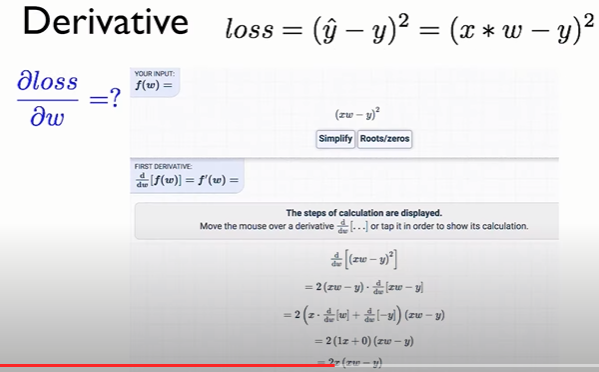
Now, given a training set, how do we pick, or learn, the parameters θ? One reasonable method seems to be to make h(x) close to y, at least for the training examples we have. To formalize this, we will define a function that measures, for each value of the θ’s, how close the h(x (i) )’s are to the corresponding y (i) ’s. We define the cost function:
We want to choose θ so as to minimize J(θ). To do so, let’s use a search algorithm that starts with some “initial guess” for θ, and that repeatedly changes θ to make J(θ) smaller, until hopefully we converge to a value of θ that minimizes J(θ).
Gradient Descent Algorithm
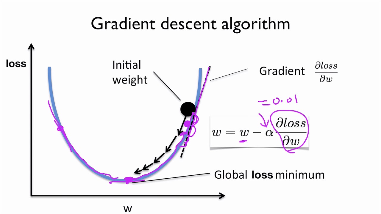
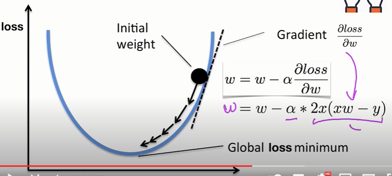
Specifically, let’s consider the gradient descent algorithm, which starts with some initial θ, and repeatedly performs the update:
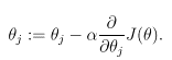
(This update is simultaneously performed for all values of j = 0, . . . , n.) Here, α is called the learning rate. This is a very natural algorithm that repeatedly takes a step in the direction of steepest decrease of J. In order to implement this algorithm, we have to work out what is the partial derivative term on the right hand side. Let’s first work it out for the case of if we have only one training example (x, y), so that we can neglect the sum in the definition of J. We have:
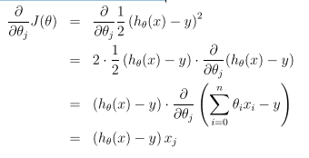
For a single training example, this gives the update rule:
Trivial code to understand how Regression works (without gradient descent algorithm)
import matplotlib.pyplot as plt
import numpy as np
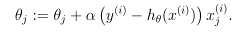
data = [[20,30], [40,50], [60,70], [90,80]]
data_x = [data[i][0] for i in range(4)]
data_y = [data[i][1] for i in range(4)]
c = 0;
errors = []
for m in np.arange(0,2,.5):
x= list(range(100))
y = [(m*x)+c for x in x]
for i in range(4):
error+= data_y[i]- (m*data_x[i]+c)
print(f'total error = {error}')
errors.append(error)
error=0
plt.plot(data_x,data_y,'r*')
plt.plot(x,y)
print(f'm = {m}')
plt.show()
print(errors)
total error = 230.0
m = 0.0
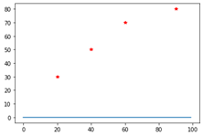
total error = 125.0
m = 0.5
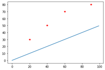
total error = 20.0
m = 1.0
total error = -85.0
m = 1.5
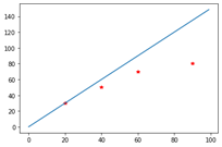
As you can see total error is minimized when m = 1. Gradient descent algorithm automatically finds the right parameters for minimum errors.