Perceptron
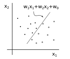
Invented in 1957 by Frank Rosenblatt at the Cornell Aeronautical Laboratory, a perceptron is the simplest neural network possible: a computational model of a single neuron. A perceptron consists of one or more inputs, a processor, and a single output.
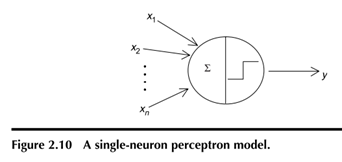
Threshold Neuron (McCulloch and Pitt’s neuron)
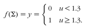
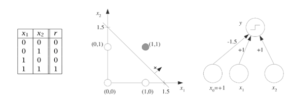
It uses the threshold function in the neuron to transform inputs to an output, producing an output of either 0 or 1. The model neuron also has fixed weights, so it does not learn. To illustrate the operation of this neuron, a simple classification problem, given in Table 2.1 and plotted in Figure 2.6a, will be solved. This problem includes two inputs (x 1 and x 2), one target output (t) that belongs to one of two categories (0 or 1), and four sets of input–output pairs. One row or one set of inputs is called an input vector or input pattern. The task is to correctly classify the input patterns into two groups (1 or 0). This task will be solved using a threshold neuron, shown in Figure 2.6b, to model the data. Here the neuron receives the two inputs through weights w 1 and w 2, but both weights will be fixed at 1.0 for this exercise, which means that there is no learning. There are two aspects to the computations in this neuron. It first calculates the net input u and then decides the output y using a threshold function. These two calculations are performed as follows: The net input u to neuron is the sum of the weighted inputs, calculated as where x 1 and x 2 are inputs. Because w 1 and w 2 are both equal to 1,
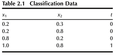
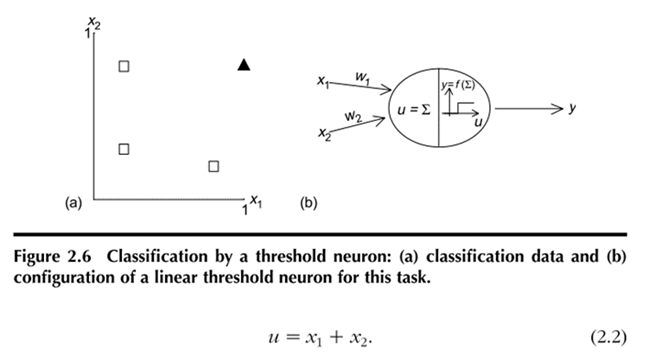
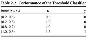
The value of u decides the activation threshold. Because the sum of the two inputs for one category is 2 and for the other category is 0, 1, and 1, respectively, for the inputs in Table 2.1, the threshold should be placed anywhere between 1.0 and 2.0. A threshold of 1.3 will be arbitrarily chosen for this case. Then the threshold function computes the activation or output (y) of the neuron as a function of u, such that
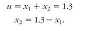
Using this simple classifier, it is now possible to check its performance. For the four inputs, the neuron output is computed following the same procedure described above; the results are presented in Table 2.2.
The neuron correctly classifies the data immediately due to the prior decision to set the threshold function at u=1.3. As stated earlier, for this case u can be fixed anywhere between 1.0 and 2.0 to obtain a correct classifier for the data. Because the location of the threshold function defines the two categories, u =1.3 decides a classification boundary that can be formulated as
This boundary line is superimposed on the data in Figure 2.7. The data on one side of the classification boundary belong to one category, and those on the other side of the boundary are classified into the other category. This is a simple classifier neuron that accumulates inputs and produces a bounded output (0 or 1) using a threshold function.
Key aspects of the above threshold neuron classifier can be summarized as follows: It does not learn from the environment (weights are equal to 1), but it can be designed to perform a classification task if the designer carefully positions the threshold function at a particular location (ideally, the neuron would decide this position by itself). The threshold neuron also classifies the data regions that are linearly separable. This means that a straight line can separate the two classes, and the threshold fixes this line as the classification boundary. Any input to the left of the boundary produces an output of 0, and those to the right of and on the boundary line yield an output of 1.
Hebbian Learning / Perceptron
A major drawback of the threshold neuron considered in the previous section is that it does not learn. In 1949, Donald Hebb, a psychologist, proposed a mechanism whereby learning can take place in neurons in a learning environment. Key points of his contribution are: He stated that the information in a network is stored in weights or connections between the neurons. He postulated that the weight change between two neurons is proportional to the product of their activation values (neuron outputs), thereby enabling a mathematical formulation of the concept that stronger excitation between neurons leads to the growth in weights between them. He proposed a neuron assembly theory, suggesting that as learning takes place by repeatedly and simultaneously activating a group of weakly connected neurons, the strength and patterns of the weights between them undergo incremental changes, leading to the formation of assemblies of strongly connected neurons. Rosenblatt proposed the first neural model, called perceptron, which was capable of learning to classify certain pattern sets as similar or dissimilar by modifying its connections. Essentially, he made threshold neurons learn using Hebbian learning. The neurons in perceptron are threshold neurons working together. However, the difference is that a perceptron network learns from example data and the weights change during learning.
Functions like AND and OR are linearly separable and are solvable using the perceptron.
The Perceptron Algorithm
- For every input, multiply that input by its weight.
- Sum all of the weighted inputs.
- Compute the output of the perceptron based on that sum passed through an activation function (the sign of the sum).
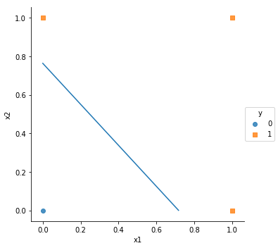
Perceptron for classifying OR function
import numpy as np
import matplotlib.pyplot as plt
import seaborn as sns
import pandas as pd
def step_function(x):
if x<0:
return 0
else:
return 1
training_set = [((0, 0), 0), ((0, 1), 1), ((1, 0), 1), ((1, 1), 1)]
# ploting data points using seaborn (Seaborn requires dataframe)
plt.figure(0)
x1 = [training_set[i][0][0] for i in range(4)]
x2 = [training_set[i][0][1] for i in range(4)]
y = [training_set[i][1] for i in range(4)]
df = pd.DataFrame(
{'x1': x1,
'x2': x2,
'y': y
})
sns.lmplot("x1", "x2", data=df, hue='y', fit_reg=False, markers=["o", "s"])
# parameter initialization
w = np.random.rand(2)
errors = []
eta = .5
epoch = 30
b = 0
# Learning
for i in range(epoch):
for x, y in training_set:
# u = np.dot(x , w) +b
u = sum(x*w) + b
error = y - step_function(u)
errors.append(error)
for index, value in enumerate(x):
#print(w[index])
w[index] += eta * error * value
b += eta*error
''' produce all decision boundaries
a = [0,-b/w[1]]
c = [-b/w[0],0]
plt.figure(1)
plt.plot(a,c)
'''
# final decision boundary
a = [0,-b/w[1]]
c = [-b/w[0],0]
plt.plot(a,c)
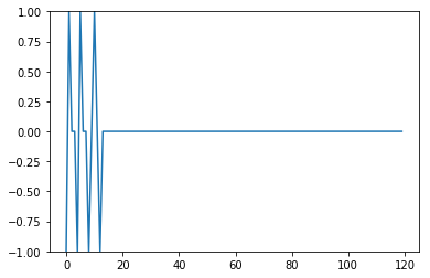
# ploting errors
plt.figure(2)
plt.ylim([-1,1])
plt.plot(errors)
Decision Boundary
Error