Bias-variance trade-off

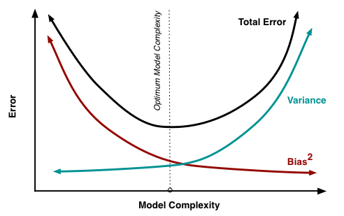
In Machine Learning, the errors made by your model is the sum of three kinds of errors — error due to bias in your model, error due to model variance and finally error that is irreducible. The following equation summarizes the sources of errors.

Total Error = Bias + Variance + Irreducible Error

Even if you had a perfect model, you might not be able to remove the errors made by a learning algorithm completely. This is because the training data itself may contain noise. This error is called Irreducible error or Bayes’ error rate or the Optimum Error rate. While you cannot do anything about the Optimum Error Rate, you can reduce the errors due to bias and variance.

When building machine learning models, we want to keep error as low as possible. Two major sources of error are bias and variance. If we managed to reduce these two, then we could build more accurate models.

It is important to note that linear regression models are susceptible to low variance/high bias, meaning that, under repeated sampling, the predicted values won’t deviate far from the mean (low variance), but the average of those models won’t do a great job capturing the true relationship (high bias). This is what’s known as the bias-variance trade-off in supervised learning, which prevents the model from generalizing beyond the training dataset.

If your machine learning model is not performing well, it is usually a high bias or a high variance problem. The figure below graphically shows the effect of model complexity on error due to bias and variance.

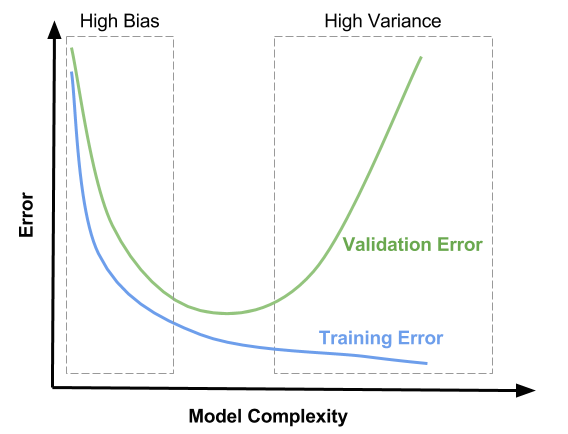
The region on the left, where both training and validation errors are high, is the region of high bias. On the other hand, the region on the right where validation error is high, but training error is low is the region of high variance. We want to be in the sweet spot in the middle.

Error due to Bias

The error due to bias is taken as the difference between the expected (or average) prediction of our model and the correct value which we are trying to predict. Of course you only have one model so talking about expected or average prediction values might seem a little strange. However, imagine you could repeat the whole model building process more than once: each time you gather new data and run a new analysis creating a new model. Due to randomness in the underlying data sets, the resulting models will have a range of predictions. Bias measures how far off in general these models’ predictions are from the correct value.

Error due to Variance

The error due to variance is taken as the variability of a model prediction for a given data point. Again, imagine you can repeat the entire model building process multiple times. The variance is how much the predictions for a given point vary between different realizations of the model.

Bias refers to the error due to overly-simplistic assumptions or faulty assumptions in the learning algorithm. Bias results in under-fitting the data. A high bias means our learning algorithm is missing important trends amongst the features.

Variance refers to the error due to an overly-complex that tries to fit the training data as closely as possible. In high variance cases the model’s predicted values are extremely close to the actual values from the training set. The learning algorithm copies the training data’s trends and this results in loss of generalization capabilities. High Variance gives rise to over-fitting

A model having high variance when tested on unseen data will not yield satisfactory results. This is because the algorithm is highly sensitive to high degrees of variation in the training data, which results in it carrying too much noise from training data for the model to be useful for the test data. \(error(X) = noise(X) + bias(X) + variance(X)\)

Over-fit & Under-fit

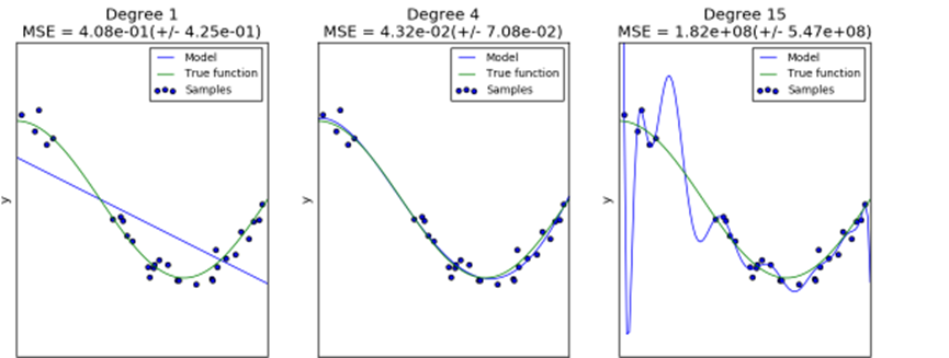
Every estimator has its advantages and drawbacks. Its generalization error can be decomposed in terms of bias, variance and noise. The bias of an estimator is its average error for different training sets. The variance of an estimator indicates how sensitive it is to varying training sets. Noise is a property of the data.

We see that the first estimator can at best provide only a poor fit to the samples and the true function because it is too simple (high bias), the second estimator approximates it almost perfectly and the last estimator approximates the training data perfectly but does not fit the true function very well, i.e. it is very sensitive to varying training data (high variance).

Bias and variance are inherent properties of estimators and we usually have to select learning algorithms and hyperparameters so that both bias and variance are as low as possible (see Bias-variance dilemma). Another way to reduce the variance of a model is to use more training data

Naive Bayes is an example of a high bias - low variance classifier (aka simple and stable, not prone to overfitting). An example from the opposite side of the spectrum would be Nearest Neighbour (kNN) classifiers, or Decision Trees, with their low bias but high variance (easy to overfit). Bagging (Random Forests) as a way to lower variance, by training many (high-variance) models and averaging.

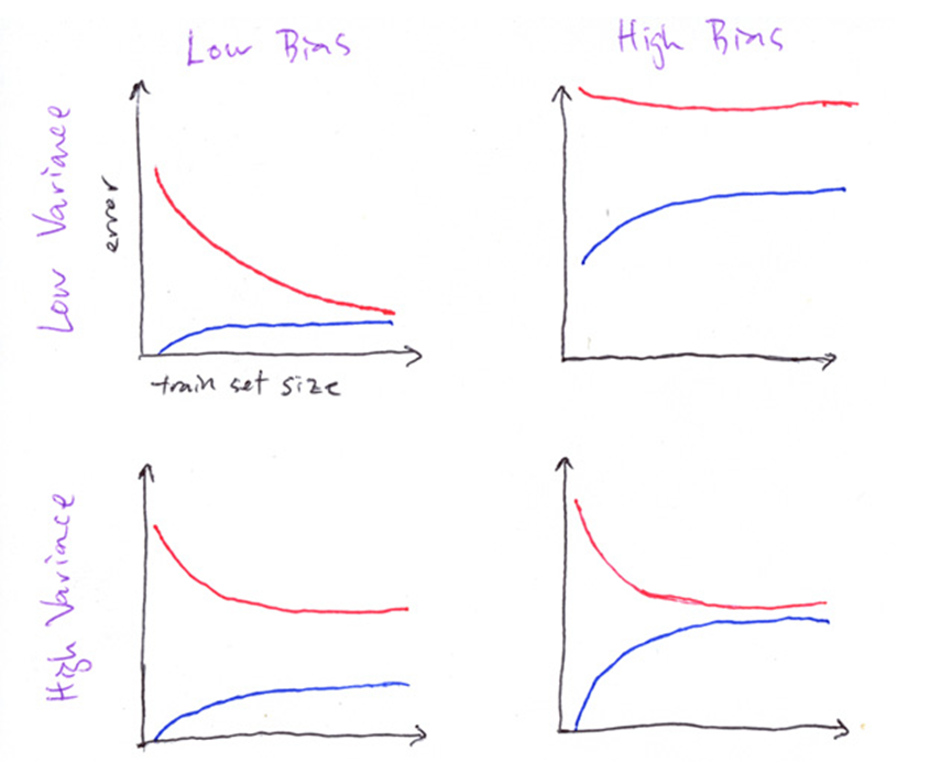
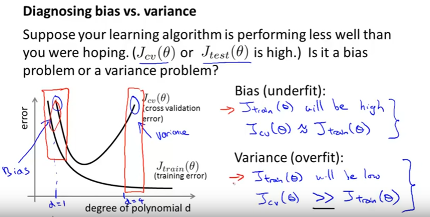
How to detect a high bias problem?

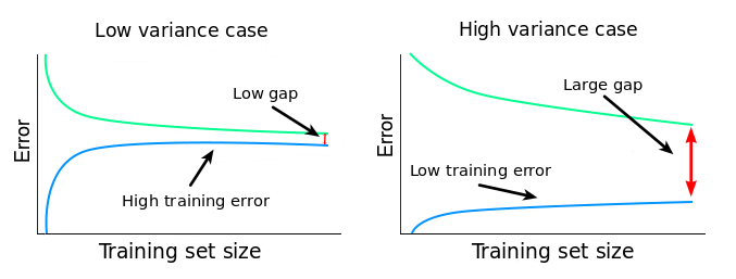
If two curves are “close to each other” and both of them but have a low score. The model suffer from an under fitting problem (High Bias). A high bias problem has the following characteristics

1. High training error.
2. Validation error is similar in magnitude to the training error.

How to detect a high variance problem?

If training curve has a much better score but testing curve has a lower score, i.e., there are large gaps between two curves. Then the model suffer from an over fitting problem (High Variance). A high variance problem on the other hand has the following characteristics

1. Low training error
2. Very high Validation error

Training set/ validation set/ test set

1. Training set (60% of the original data set): This is used to build up our prediction algorithm. Our algorithm tries to tune itself to the quirks of the training data sets. In this phase we usually create multiple algorithms in order to compare their performances during the Cross-Validation Phase.
2. Cross-Validation set (20% of the original data set): This data set is used to compare the performances of the prediction algorithms that were created based on the training set. We choose the algorithm that has the best performance.
3. Test set (20% of the original data set): Now we have chosen our preferred prediction algorithm but we don’t know yet how it’s going to perform on completely unseen real-world data. So, we apply our chosen prediction algorithm on our test set in order to see how it’s going to perform so we can have an idea about our algorithm’s performance on unseen data.

• the training set is used to train a given model
• the validation set is used to choose between models (for instance, does a random forest or a neural net work better for your problem? do you want a random forest with 40 trees or 50 trees?)
• the test set tells you how you’ve done. If you’ve tried out a lot of different models, you may get one that does well on your validation set just by chance, and having a test set helps make sure that is not the case.

Training/ testing error

Training error is the error that you get when you run the trained model back on the training data. Remember that this data has already been used to train the model and this necessarily doesn’t mean that the model once trained will accurately perform when applied back on the training data itself.

Test error is the error when you get when you run the trained model on a set of data that it has previously never been exposed to. This data is often used to measure the accuracy of the model before it is shipped to production.

Learning Curve

A learning curve shows the relationship of the training score vs the cross validated test score for an estimator with a varying number of training samples. This visualization is typically used two show two things:

1. How much the estimator benefits from more data (e.g. do we have “enough data” or will the estimator get better if used in an online fashion).
2. If the estimator is more sensitive to error due to variance vs. error due to bias.

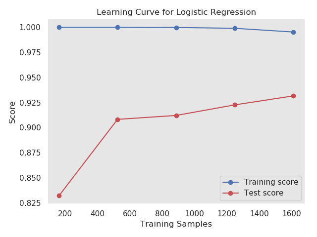
Drawing Learning Curve

Using built-in learning_curve() function from sklearn module we can easily draw learning curve.

import numpy as np
import matplotlib.pyplot as plt
from sklearn.model_selection import learning_curve
from sklearn.datasets import load_digits
from sklearn.naive_bayes import GaussianNB
from sklearn.linear_model import LogisticRegression

digit = load_digits()
X, y = digit.data, digit.target

#model = GaussianNB()
model = LogisticRegression()

train_size, train_score, test_score = learning_curve(estimator=model, X=X, y=y, cv=10 )

train_score_m = np.mean(train_score, axis=1)
test_score_m = np.mean(test_score, axis=1)

plt.plot(train_size, train_score_m, 'o-', color="b")
plt.plot(train_size, test_score_m, 'o-', color="r")
plt.legend(('Training score', 'Test score'), loc='best')
plt.xlabel("Training Samples")
plt.ylabel("Score")
plt.title("Learning Curve for Logistic Regression")
plt.grid()

plt.show()

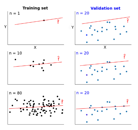
Let’s say we have some data and split it into a training set and validation set. We take one single instance (that’s right, one!) from the training set and use it to estimate a model. Then we measure the model’s error on the validation set and on that single training instance. The error on the training instance will be 0, since it’s quite easy to perfectly fit a single data point. The error on the validation set, however, will be very large. That’s because the model is built around a single instance, and it almost certainly won’t be able to generalize accurately on data that hasn’t seen before.

Now let’s say that instead of one training instance, we take ten and repeat the error measurements. Then we take fifty, one hundred, five hundred, until we use our entire training set. The error scores will vary more or less as we change the training set.

We thus have two error scores to monitor: one for the validation set, and one for the training sets. If we plot the evolution of the two error scores as training sets change, we end up with two curves. These are called learning curves.

In the first row, where n = 1 (n is the number of training instances), the model fits perfectly that single training data point. However, the very same model fits really bad a validation set of 20 different data points. So the model’s error is 0 on the training set, but much higher on the validation set.

As we increase the training set size, the model cannot fit perfectly anymore the training set. So the training error becomes larger. However, the model is trained on more data, so it manages to fit better the validation set. Thus, the validation error decreases. To remind you, the validation set stays the same across all three cases.

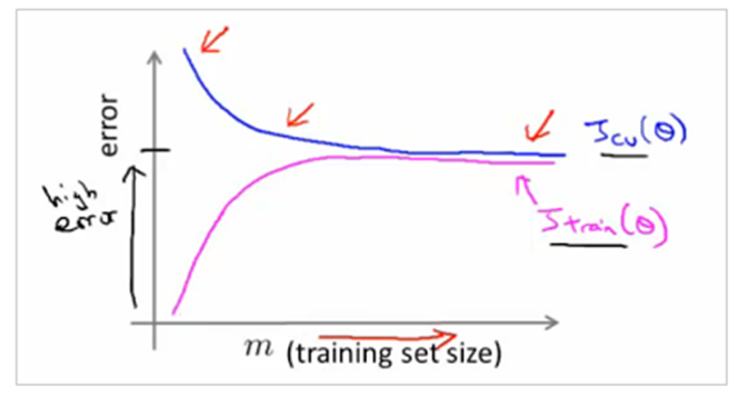
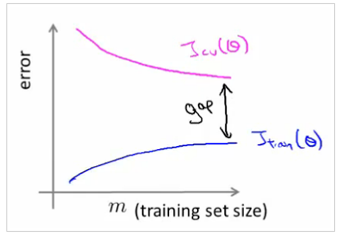
If we plotted the error scores for each training size, we’d get two learning curves looking similarly to these:

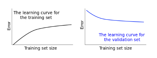
Learning curves give us an opportunity to diagnose bias and variance in supervised learning models.

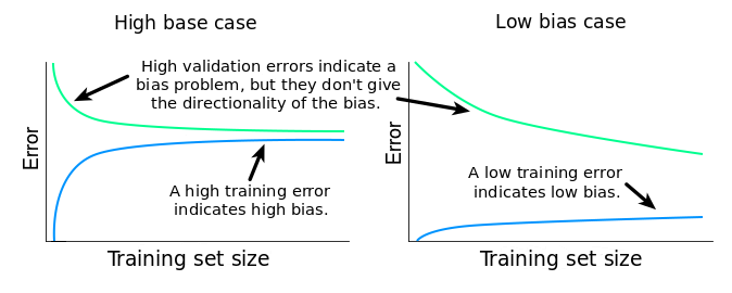
If the training error is high, it means that the training data is not fitted well enough by the estimated model. If the model fails to fit the training data well, it means it has high bias with respect to that set of data.

variance

A narrow gap indicates low variance. Generally, the more narrow the gap, the lower the variance. The opposite is also true: the wider the gap, the greater the variance.

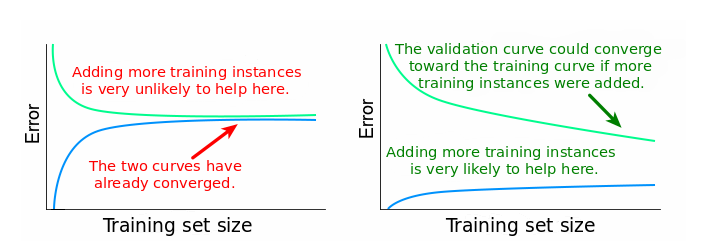
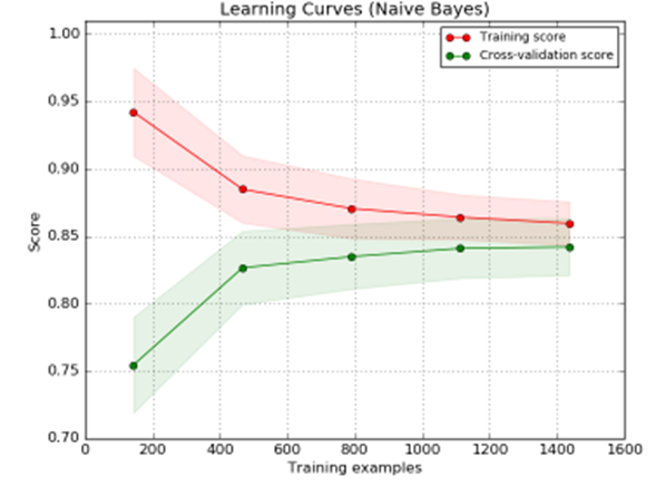
A learning curve shows the validation and training score/ error of an estimator for varying numbers of training samples. It is a tool to find out how much we benefit from adding more training data and whether the estimator suffers more from a variance error or a bias error. If both the validation score and the training score converge to a value that is too low with increasing size of the training set, we will not benefit much from more training data. In the following plot you can see an example: naive Bayes roughly converges to a low score.

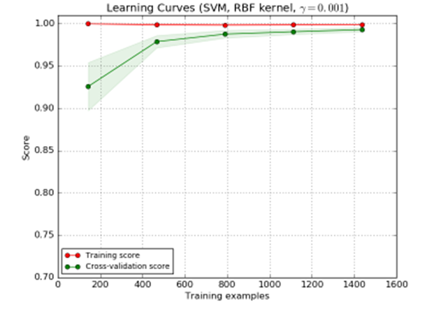
We will probably have to use an estimator or a parametrization of the current estimator that can learn more complex concepts (i.e. has a lower bias). If the training score is much greater than the validation score for the maximum number of training samples, adding more training samples will most likely increase generalization. In the following plot you can see that the SVM could benefit from more training examples.

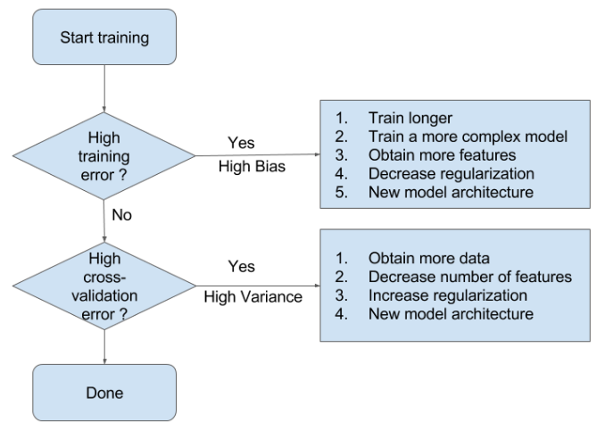
Fixing High Bias

• When training and testing errors converge and are high
• No matter how much data we feed the model, the model cannot represent the underlying relationship and has high systematic error
• Poor fit
• Poor generalization

A high bias model has few parameters and may result in underfitting. Essentially we’re trying to fit an overly simplistic hypothesis, for example linear where we should be looking for a higher order polynomial. In a high bias situation, training and cross-validation error are both high and more training data is unlikely to help much.

• find more features
• add polynomial features
• increase parameters (more hidden layer neurons, for example)
• decrease regularization

Fixing High variance

• When there is a large gap between the errors
• Require data to improve
• Can simplify the model with fewer or less complex features

Variance is the opposite problem, having lots of parameters, which carries a risk of overfitting. If we are overfitting, the algorithm fits the training set well, but has high cross-validation and testing error. If we see low training set error, with cross-validation error trending downward, then the gap between them might be narrowed by training on more data.

• more training data
• reduce number of features, manually or using a model selection algorithm
• increase regularization

Why does the training accuracy start so high, then suddenly drop?

It is normal that your training accuracy goes down when the dataset size grows. Think of it this way: when you have fewer samples (imagine that you have just one, at the extreme) it is easy to fit a model that has good accuracy for the training data, however that fitted model is not going to generalize well for test data. As you increase the dataset size, in general it is going to be harder to fit the training data, but hopefully your results generalize better for the test data.

The Trade-Off

There is no escaping the relationship between bias and variance in machine learning.

• Increasing the bias will decrease the variance.
• Increasing the variance will decrease the bias.

There is a trade-off at play between these two concerns and the algorithms you choose and the way you choose to configure them are finding different balances in this trade-off for your problem

In reality, we cannot calculate the real bias and variance error terms because we do not know the actual underlying target function. Nevertheless, as a framework, bias and variance provide the tools to understand the behavior of machine learning algorithms in the pursuit of predictive performance.

Below are two examples of configuring the bias-variance trade-off for specific algorithms:

• The k-nearest neighbors algorithm has low bias and high variance, but the trade-off can be changed by increasing the value of k which increases the number of neighbors that contribute t the prediction and in turn increases the bias of the model.
• The support vector machine algorithm has low bias and high variance, but the trade-off can be changed by increasing the C parameter that influences the number of violations of the margin allowed in the training data which increases the bias but decreases the variance.